Grand Forest • Unsupervised workflow user guide
Contents
1. Expression data format
Expression data must be uploaded as a data table in one of the formats described on the expression data file format page.
Including known clusters
Known clusters can be included with the expression data for visualization purposes. These clusters will not affect the model training, but are used for annotation in heatmaps and the split tree.
In order to include known clusters add an additional column containing class labels to the data file. The column can have any name as long as it is unique. Example of a table with known subtype information in first column:
| subtype | 2099 | 351 | 7534 | 8452 |
|---|---|---|---|---|
| lumA | 0.40 | 0.50 | 0.88 | 0.81 |
| lumA | 0.42 | 0.95 | 0.31 | 0.15 |
| lumB | 0.91 | 0.99 | 0.88 | 0.57 |
| lumB | 0.72 | 0.19 | 0.32 | 0.16 |
| her2 | 0.19 | 0.85 | 0.03 | 0.37 |
| her2 | 0.97 | 0.78 | 0.96 | 0.18 |
Including survival information
Survival information can also be included to enable survival analysis. In order to include survival information two additional columns must be added to the data file:
- A survival time column containing numeric values.
- An event/status column containing either
1(event) or0(no event).
Example of a table containing survival information:
| status | time | 2099 | 351 | 7534 | 8452 |
|---|---|---|---|---|---|
| 1 | 1.03 | 0.40 | 0.50 | 0.88 | 0.81 |
| 0 | 7.12 | 0.42 | 0.95 | 0.31 | 0.15 |
| 1 | 0.21 | 0.91 | 0.99 | 0.88 | 0.57 |
| 1 | 3.10 | 0.72 | 0.19 | 0.32 | 0.16 |
| 0 | 5.45 | 0.19 | 0.85 | 0.03 | 0.37 |
| 1 | 4.93 | 0.97 | 0.78 | 0.96 | 0.18 |
2. Uploading data
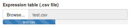
In order to start the analysis, we first need to upload a data file containing the expression data. The data file should be formatted as described above. Once a file has been selected the upload will start automatically.
Next we need to choose the network data source we want to use. We can either use one of the available networks or choose Custom network to upload our own network file (see network file format for details.) Here we will use experimentally validated interactions from the IID database.
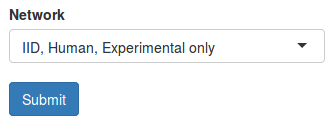
Once a network is chosen and the file is done uploading, click Submit to continue.
Using the example data set
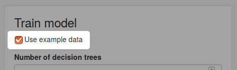
An example data set is also provided for demonstration. To use the example data, simply check the Use example data option from the sidebar.
The data set contains RNA-seq data from 947 breast cancer samples obtained from the TCGA-BRCA project that were classified as either the Luminal A or Luminal B subtype using the PAM50 gene signature. The example data also include survival information and the PAM50 subtype classifications.
3. Splitting the data
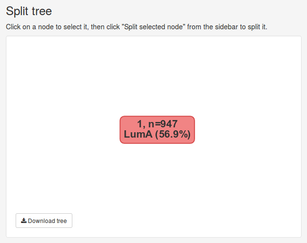
Once the data has been submitted, we will be presented with several new panels. The Split tree panel visualizes our hierarchical clustering of the data set as a tree. Currently we only have cluster containing 947 samples, visualizes by the the single red node. Nodes can be selected by clicking on them and deselected by clicking the white space around them. The currently selected node will be colored red.
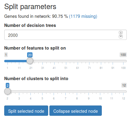
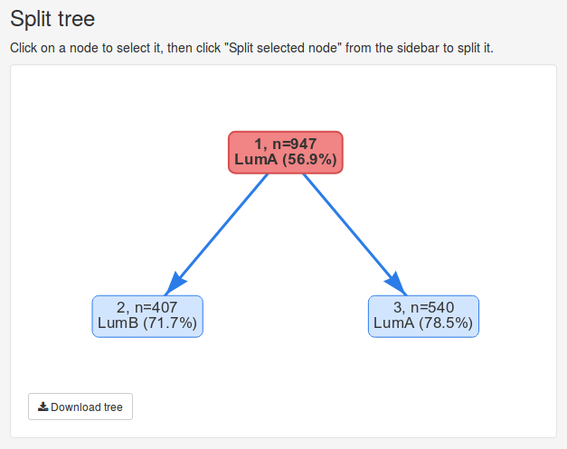
We can split the currently selected node using the tools in the sidebar under Split parameters.
- Under Number of decision trees we can choose how many trees we want to train when performing the split. Increasing the number of trees will increase the model’s stability but also the necessary computation time.
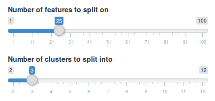
- Under Number of features to split on we can choose how many features we want to use for splitting the node.
- Under Number of clusters to split into we need to choose how many clusters we want to split this node into.
In this example we will use 20 features to split the root node into 2 clusters. Click Split selected node to split the data. Once the split is complete, the split tree will now contain two new nodes representing the clusters we created. We can observe that the two new clusters contain 407 and 540 samples, respectively. If the data set contains known cluster information the nodes will also show the most common known cluster label in each cluster and the percentage of samples with that label. Here we observe that one cluster consists of 71.7% Luminal B samples while the other cluster consists of 78.5% Luminal A samples.
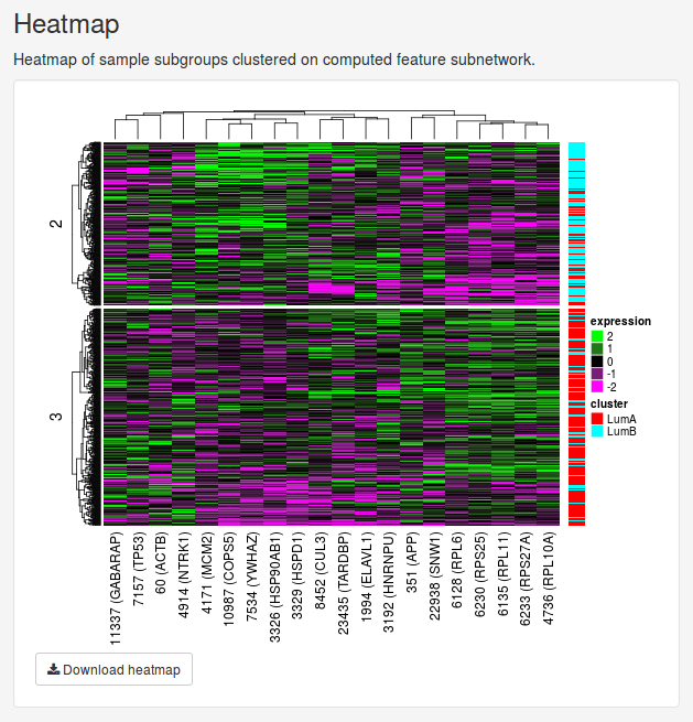
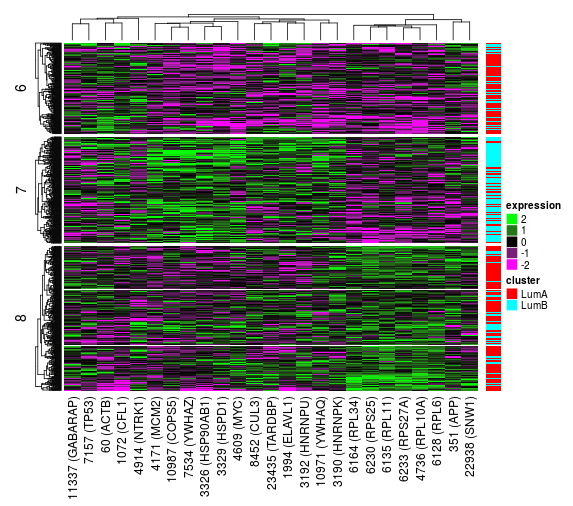
When a split node (non-leaf node) is selected, the features used for splitting will be visualized as a heatmap and an interaction network.
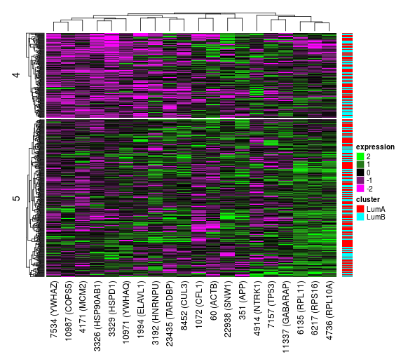
The Heatmap panel shows the expression of all patients in the selected node for only the features selected for splitting. The samples will be grouped into the clusters they have been split into. If the data set includes known cluster data, these clusters will by shown as a color annotation to the right to the right of the heatmap as well.
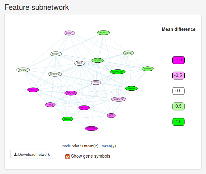
The Feature subnetwork is constructed by extracting all the genes selected for splitting along with all the interactions between them in the interaction network we chose in the beginning. If the node is only split into two clusters, the nodes will also be colored according to the difference in mean expression between these two groups.
We might suspect that one of the clusters actually consists of several subgroups. In order to split the data set further, we need to select one of the leaf nodes and split it using the controls in the side bar. As an example let’s select cluster 3 and split it into two futher clusters. Once the split is complete, the split tree will now contains two split nodes (node 1 and 3) and three leaf nodes (2, 4 and 5). If we select node 3 we will be presented with a new heatmap showing the expression for the samples in the two new clusters.
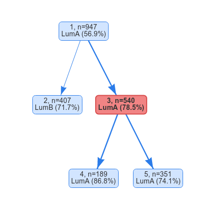
If we want to change the change the number of split features and number of clusters for a split we can do so simply by selecting an already split node, changing the parameters and hitting Split selected node again. Let’s try and split the root node into 3 clusters instead using 25 features.
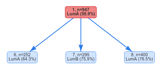
Survival analysis
If the data set contains survival information we can compare survival curves of the produced clusters. Under Survival analysis we see a Kaplan-Meier plot for the two clusters we created. The provided p-value is computed using a log-rank test. If the data set also includes known clusters, we can compare the survival curves of our clustering to the a priori clusters by enabling the Plot known clusters option. Here we observe that the de novo classification we computed (left) provides a more significant stratification than the PAM50 classification (right) with respect to distant metastasis free survival.
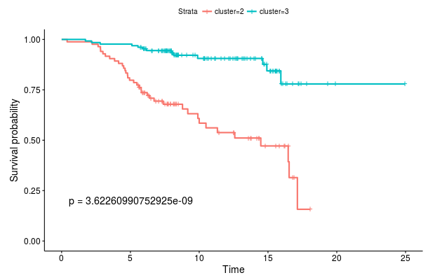 Survival curves for root node splits
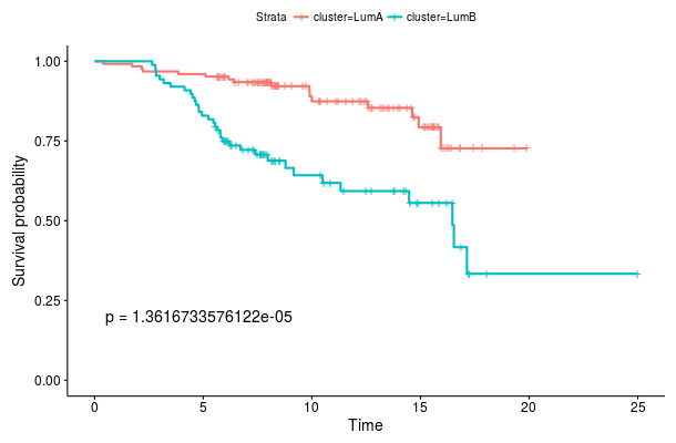 Survival curves for Luminal A and Luminal B classification
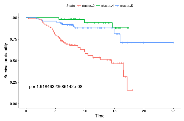
If we instead select All leaf nodes above the plots, we can choose to show all leaf nodes in the tree. In this case we performed two splits resulting in three leaf nodes so we get three survival curves. However, we observe that the two new clusters (4 and 5) do not appear to have significantly different survival functions.
4. Gene set enrichment
Once we have found an interesting gene subnetwork that appears to split our dataset well, we can investigate whether these genes are significantly overrepresented in some GO terms, pathways or diseases. In order to perform gene set enrichment, first we need to select a split node to investigate. In this case we will select the root node. Then we must select the Gene set enrichment tab above the feature table.
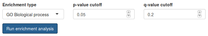
Under Enrichment type we can select which source of gene sets we want to check for enrichment. Here we select GO Biological process. The p-value cutoff and q-value cutoff parameters are used to filter results. Only gene sets with p- and q-value below these cutoffs will be reported.
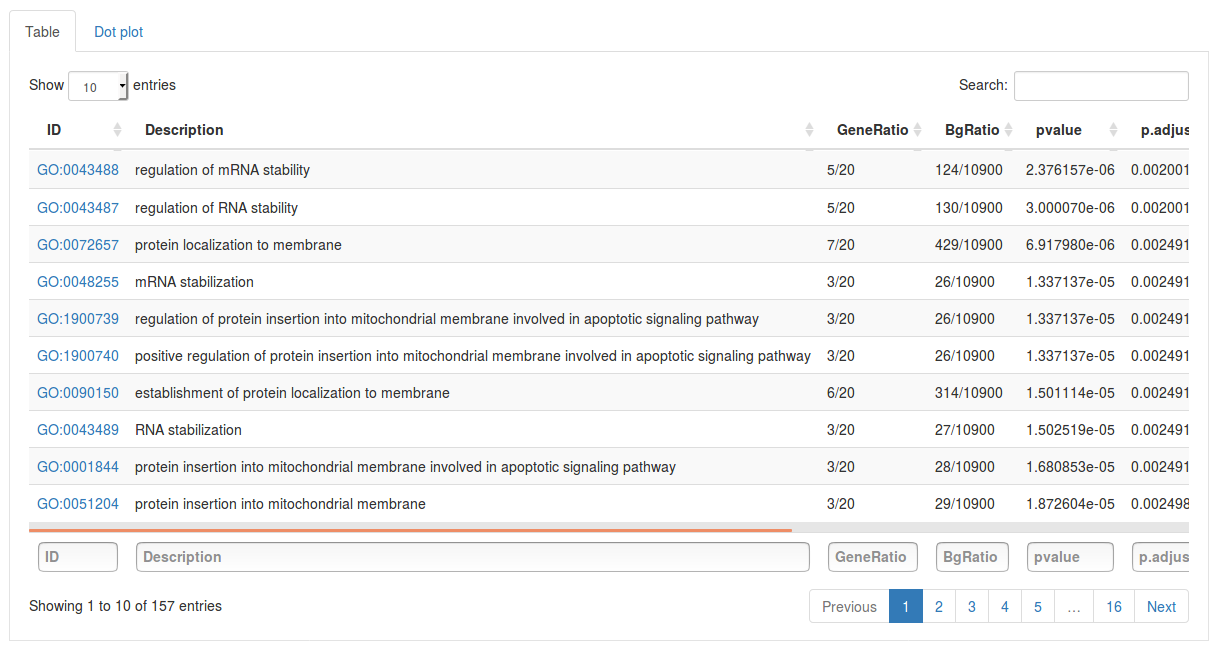
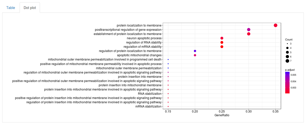
Click Run enrichment analysis to run the enrichment. After a little while a table will show up with all significantly enriched gene sets, ordered by p-value. For each gene set the table will show the name of the gene set (in this case GO term), how many genes in our subnetwork were actually found in that gene set, as well as a p-value, adjusted p-value and q-value. The search fields above the table can be used to search for specific gene sets. By selecting the Dot plot tab above the table we can also visualize the top results using a dot plot.
5. Finding drug and miRNA targets
We can also search for drugs and miRNAs targeting our genes of interest. First, select the Gene targets tab under Genes.
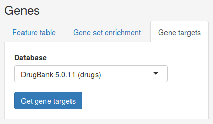
Under database we can choose the source database we want to search in. Here we select the DrugBank database to search for drugs targeting our genes. Once you have selected a database click Get gene targets to start the search. The found targets will appear in a table below.
Each row in the table contains a gene and a drug targeting it. Click on the drug ID of a drug to open its page on the DrugBank website. Other columns will also link to external databases such as PubChem and KEGG if available. Using the search fields below the columns we can also filter the results by gene or drug name.
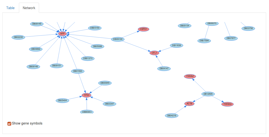
If we select the Network tab above we table we can also visualize the drug targets as a network. Here, each red node corresponds to a gene of interest and and each blue node corresponds to a drug.